
Applied Maths
the maths isn't too difficult
The greatest shortcoming of the human race is our inability to understand the exponential function. (Prof. Al Bartlett)
Exponential problems are difficult for our mind to understand, because we tend to think linear rather than exponential.
The maths used on this site to analyse the corona virus outbreak is not too difficult. The applied models for fits and predictions of data are rather simple models, just because to have very few parameters to fit and therefore get more accurate fitting results. In complex models, some parameters are not as independent as needed for the least square method.
Your support will help us working on new data analyis on Covid-19 for you:

(by click on image you accept third party cookies, required by paypal.)
Exponential growth
A very simple growth model is given by:
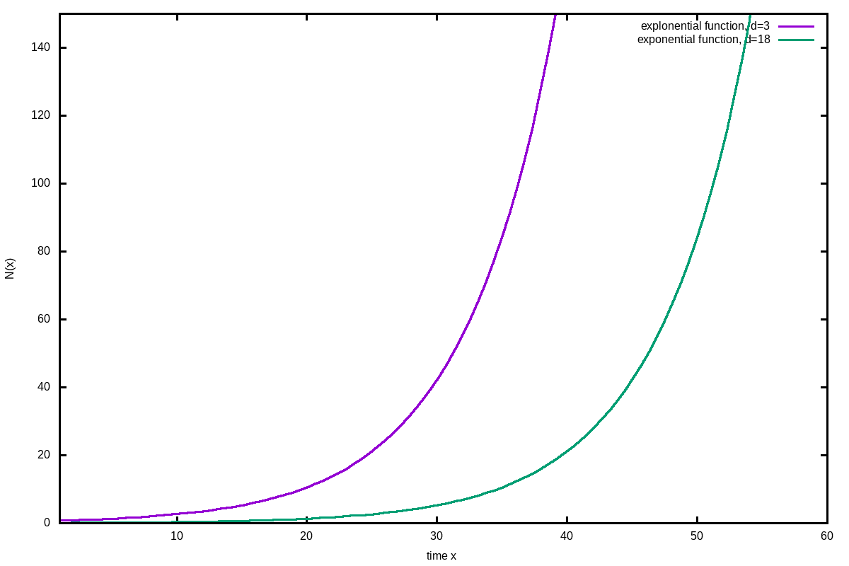
\[ N(x) = N_0\cdot e^{\frac{ln(2)}{T_2} (x-d)} \]
Hereby is:
e: Euler’s number 2.71828182845905…
N0: the number of organisms or cases at time zero
N(x): the number at time x
x: the time counter, which can be seconds, minutes, hours, days, years
d: the shift of the function in x-axis by d time counters
T2: the doubling time in unit of x.
In real data the starting point might not be at zero. Therefore, the function needs to be shifted along the x-axis without being altered in its shape, which is achieved by the d parameter. If d is positive, the function wills shift to the right. However, N0 and d are not fully independent and will cause trouble, when data are fitted by the least square method. The results are very large error values. Therefore only one of those values can be fitted and the other requires a good estimate. If in most cases N0 is known, the beginning of a growth can be calculated, e.g. when N0=1, then N(x) is crossing the value 1, (x-d) will tell the time.
This simple function is useful especially in the beginning of a natural growth, when no limitations hinder the growth. The most important value we obtain is the doubling time, which tells the speed of growth.
Doubling times are useful to be simply calculated in mind:
\[ N = N_0\cdot 2\cdot 2\cdot 2\cdot 2 … \]
or
\[ N = N_0 \cdot 2^n \]
with n the number of doubling. In order to calculate the time for n doubling:
\[ time = T_2 \cdot n \]
This simple maths can be easily done without a calculator. It just shows, how quick numbers can rise. Lets do a practical example and assume, the doubling time T2=3 days and we run n=32 doubling by N0=1. The number N is:
\[ N = 1 \cdot 2^{32} = 4,294,967,296 \]
This would be a bit more than half the population of the earth in 32 steps. The next doubling will already be twice that number. How long will it take:
\[ time = 3 \cdot 32\ days = 96\ days \]
It took about 3 months to reach half the population. How long will it take to reach from half the population to all the population: 1 doubling time: 3 days!
If we assume 0.2% of the population is infected, then show much time is left until everybody will be? The answer is about 9 doubling times or about 4 weeks.
When is it time to act by exponential growth problems? In the beginning!
Logistic function

The simple exponential growth function can only be used in the beginning of a growth process. In natural conditions the number of possible expandable space or victims for viruses is limited. When the limitation starts to act, the expansion is slowed and approaches the limit. It can be described by:
Hereby are the parameters the same as for the exponential growth
and have additionally:
Nmax: maximum N that is possible.
The function has the form of a symmetric S shape. The doubling time T2 shows the rise in the beginning and the asymptotic declining at the end. During the transition there is a characteristic linear phase with a turning point.
Once the turning point is crossed, fits may produce quite accurate Nmax results. However, in reality, natural growths have different shapes and a longer declining phase. Therefore this function should only be used in the beginning as a more advance replacement of the exponential function, as we can set Nmax to the realistic limit and obtain a better prediction for the next days.
Gompertz function
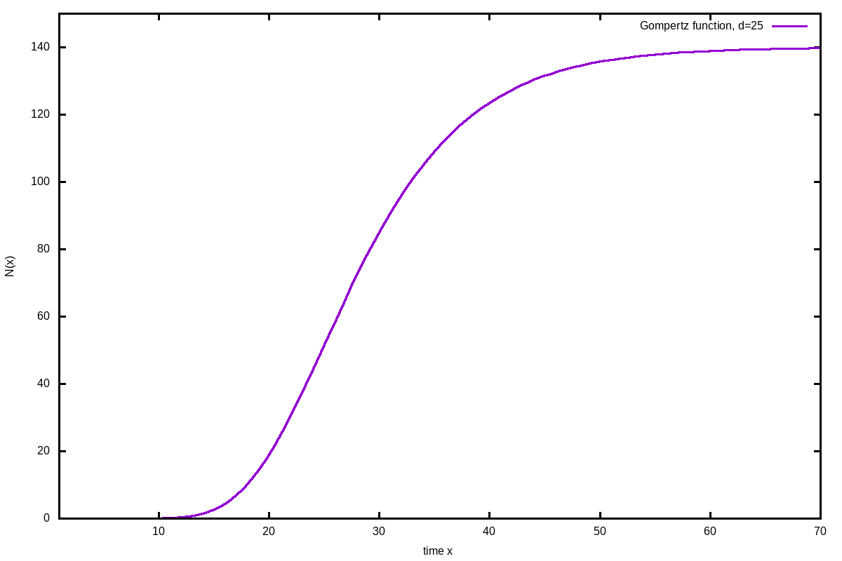
Benjamin Gompertz has described a double exponential formula to describe naturally observed growths:
\[ N(x) = N_{max}\cdot e^{-b\cdot e^{-c\cdot x}} \]
Hereby is:
b: displacement along the x-axis (abstract value)
c: growth rate (abstract value)
There are meanwhile many variations of this formula in use that are described in the literature below.
When using this formula for fitting, the least square matrix will also result in large error values because b an c in the exponent are not as independent as needed. Therefore, I have used a more simplified version, that provides very robust fits with meaningful results:
\[ N(x) = N_{max}\cdot e^{-e^{-ln(2)/T_2\cdot (x-d)}} \]
Hereby is:
Nmax: the asymptotic maximal number of cases
T2: the doubling time at the turning point
d: the direct time of the turning point!
We have therefore very important variables to evaluate the process of a growth. Especially important is the time of the turning point, because it will tell us, when we are getting e.g. an epidemic under control. Only after the turning point, the numbers of daily new infections are going to become smaller. However, till the end of process, there is still a lot time to go, because at the turning point we have only passed about 37% of the function in number of cases! Even worse, at the turning point we have roughly passed only 20% of the time till the end.
T2 describes the doubling time of the turning point and quite well as well as the asymptotic approach time. The only disadvantage of this function is that it does not tell the doubling time in the beginning of that growth. Modern versions with two doubling times do not provide stable fits and therefore, on this site, this modified simple form is used. How well it describes the growth, can be studied by the Ebola Data. There you can also see the two different doubling times in the first and second part, which were adjusted with the logistic function, but only limited to the turning point each.
This modified Gompertz function is not very accurate at the beginning of a growth, when we are far away from the turning point. It is very sensitive to small changes. The lack of seeing doubling time at this early phase may lead to misinterpretation especially in T2 that should not be mixed up with the doubling time at the quick rise phase. Using at this stage the logistic function, is recommended, which may overestimate here Nmax. Once we get near the turning point, the accuracy of the Gompertz functions becomes quite well, while the logistic function tends to underestimate Nmax.
Please be aware, that all the models assume that basic conditions do not change and a process will behave as theoretically assumed. That is not the case, as new treatments change parameters for the good of people, a behavioural change changes the doubling time of an exponential infection curve or new methods of investigations boost parameters. Neverthless, from general tendencies we can learn a lot, how long processes will take and when to act.
Usually, in exponential problems we should act as early as possible, see talk from Al Bartlett about exponential growth.
Adanced Gompertz function
In the publication below are several advance models that are especially modificing the ratio between the two parts before and after the turning point. However, most of those approaches may work fine, they are not stable in the least squared methods, leading by additional parameters often to extreme unrealistic error values. The reason is that those parameters are not sufficiently independent and therefore destabilising the fit. Here, I suggest another method, that compensates these problems and provides stable fits:
\[ N(x) = N_{max}\cdot e^{-e^{-(ln(2^{1/w})/(T_2\cdot w^{1/w}))^w\cdot (x^w-d^w)}} \]
In easier readable form:
\[ N(x) = N_{max}\cdot e^{-e^-G} \]
\[ G=(\frac{ln(2^{1/w})}{(T_2\cdot w^{1/w})})^w\cdot (x^w-d^w)\]
The advantage of that modification is, that we keep all our previously important information: T2 as the doubling time in the turning point, d as the turning point.
Literature
.·.